17. Forward Kinematics
Forward Kinematics
Congratulations! You have almost made it to the end of this lesson. Best of all, you have already seen everything you need to know to solve the forward kinematics (FK) problem for a serial manipulator. Putting it all together is going to be a piece of cake.
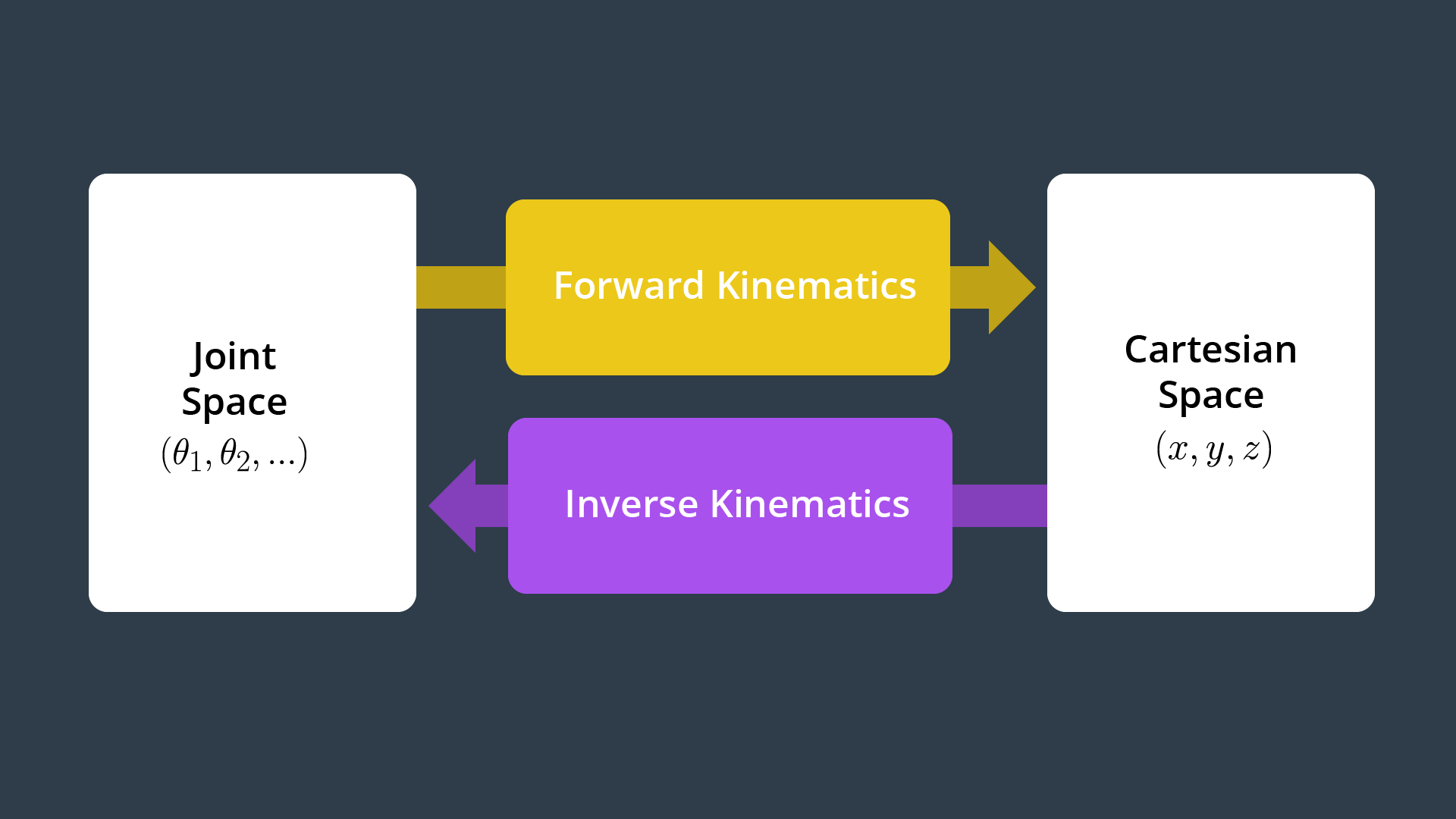
Recall that, in the FK problem, we know all the joint variables, that is the generalized coordinates associated with the revolute and prismatic joints, and we wish to calculate the pose of the end effector in a 3D world. In the next lesson we consider the more challenging inverse kinematics problem. In the IK problem the position and orientation of the end effector is known and the objective is to solve for the joint variables.
The FK problem boils down to the composition of homogeneous transforms. We start with the base link and move link by link to the end effector. And we use the DH parameters to build each individual transform.
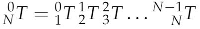
Recall that the total transform between adjacent links,
for each link is actually composed of four individual transforms, 2 rotations and 2 translations, performed in the order shown here
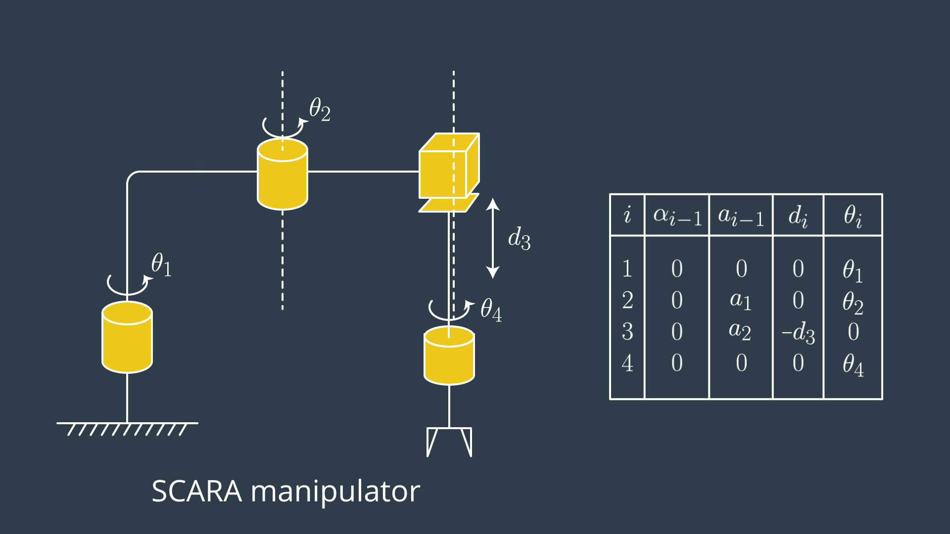
The robot we will use as an example is one we have seen before, the SCARA. You can find the DH parameter table for it in the text.
We start by importing several components from SymPy.
from sympy import symbols, cos, sin, pi, simplify
from sympy.matrices import Matrix
Next, we define symbols that we will use in the transform equations. Here I have used q’s to denote generalized coordinates; the d’s, a’s, and, alpha’s are the other DH parameters.
### Create symbols for joint variables
q1, q2, q3, q4 = symbols('q1:5')
d1, d2, d3, d4 = symbols('d1:5')
a0, a1, a2, a3 = symbols('a0:4')
alpha0, alpha1, alpha2, alpha3 = symbols('alpha0:4')
For the non-zero constant DH-parameters, I choose numerical values.
a12 = 0.4500 # meters
a23 = 0.3000 # meters
Here I set up a dictionary that binds numerical values to those DH parameters that are constants.
# DH Parameters
s = {alpha0: 0,  a0:   0, d1: 0,
     alpha1: 0,  a1: a12, d2: 0,
     alpha2: 0,  a2: a23,        q3: 0,
     alpha3: 0,  a3:   0, d4: 0}
I then define the homogeneous transform between adjacent links and, with the subs method, substitute our known constant values into the expression.
#### Homogeneous Transforms
T0_1 = Matrix([[             cos(q1),            -sin(q1),            0,              a0],
               [ sin(q1)*cos(alpha0), cos(q1)*cos(alpha0), -sin(alpha0), -sin(alpha0)*d1],
               [ sin(q1)*sin(alpha0), cos(q1)*sin(alpha0),  cos(alpha0),  cos(alpha0)*d1],
               [                   0,                   0,            0,               1]])
T0_1 = T0_1.subs(s)

T1_2 = Matrix([[             cos(q2),            -sin(q2),            0,              a1],
               [ sin(q2)*cos(alpha1), cos(q2)*cos(alpha1), -sin(alpha1), -sin(alpha1)*d2],
               [ sin(q2)*sin(alpha1), cos(q2)*sin(alpha1),  cos(alpha1),  cos(alpha1)*d2],
               [                   0,                   0,            0,               1]])
T1_2 = T1_2.subs(s)

T2_3 = Matrix([[             cos(q3),            -sin(q3),            0,              a2],
               [ sin(q3)*cos(alpha2), cos(q3)*cos(alpha2), -sin(alpha2), -sin(alpha2)*d3],
               [ sin(q3)*sin(alpha2), cos(q3)*sin(alpha2),  cos(alpha2),  cos(alpha2)*d3],
               [                   0,                   0,            0,               1]])
T2_3 = T2_3.subs(s)

T3_4 = Matrix([[             cos(q4),            -sin(q4),            0,              a3],
               [ sin(q4)*cos(alpha3), cos(q4)*cos(alpha3), -sin(alpha3), -sin(alpha3)*d4],
               [ sin(q4)*sin(alpha3), cos(q4)*sin(alpha3),  cos(alpha3),  cos(alpha3)*d4],
               [                   0,                   0,            0,               1]])
T3_4 = T3_4.subs(s)
Finally, I create the overall transform between the base frame and end effector by composing the individual link transforms.
# Transform from base link to end effector
T0_4 = simplify(T0_1 * T1_2 * T2_3 * T3_4)
As the name suggests, simplify attempts to simplify the expression by making use of trigonometric identities and canceling or factoring common terms whenever possible.
The print command displays the overall transform.
print(T0_4)There are many ways to numerically evaluate a symbolic expression, a simple one is to use the evalf method and pass in a dictionary.
print(T0_4.evalf(subs={q1: 0, q2: 0, d3: 0, q4: 0}))Before I show you the output, see if you can guess what the general form of this homogeneous transform between the base and end effector should look like. Look at how the reference frames are attached to each link in this "zero" joint-variable configuration.
Test Your Intuition
SOLUTION:
Matrix([[1, 0, 0], [0, 1, 0], [0, 0, 1]])Executing the code from above gives,
Matrix([
[1.0,   0,   0, 0.75],
[  0, 1.0,   0,    0],
[  0,   0, 1.0,    0],
[  0,   0,   0,  1.0]])
(X,Y,Z) Coordinates of end effector
SOLUTION:
(X,Y,Z) = (0.75, 0, 0)Now evaluate the homogeneous transform when q_1 = q_2 = q_4 = 0 and d_3 = -0.5 . In this case, the rotational component of the homogeneous transform should not change, only the Z-coordinate should. Printing the output gives,
Matrix([
[1.0,   0,   0, 0.75],
[  0, 1.0,   0,    0],
[  0,   0, 1.0, -0.5],
[  0,   0,   0,  1.0]])
matching our expectations.